The German Tank Problem

Sometimes I stumble upon fascinating instances of math being directly applicable in the history of warfare that doesn't involve the creation of weapons or technology. The World War II Enigma code, its workings, and its subsequent breaking by Polish and British cryptographers is a great example, especially if you have a knack for diabolically clever electrical circuitry and very large numbers. The German Tank Problem is a simpler such example, involving some probability instead.

The German Tank

To appreciate why this was an actual problem, we need to look at a tiny bit of World War II history.

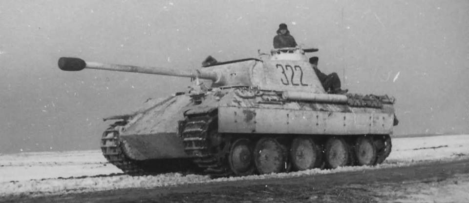
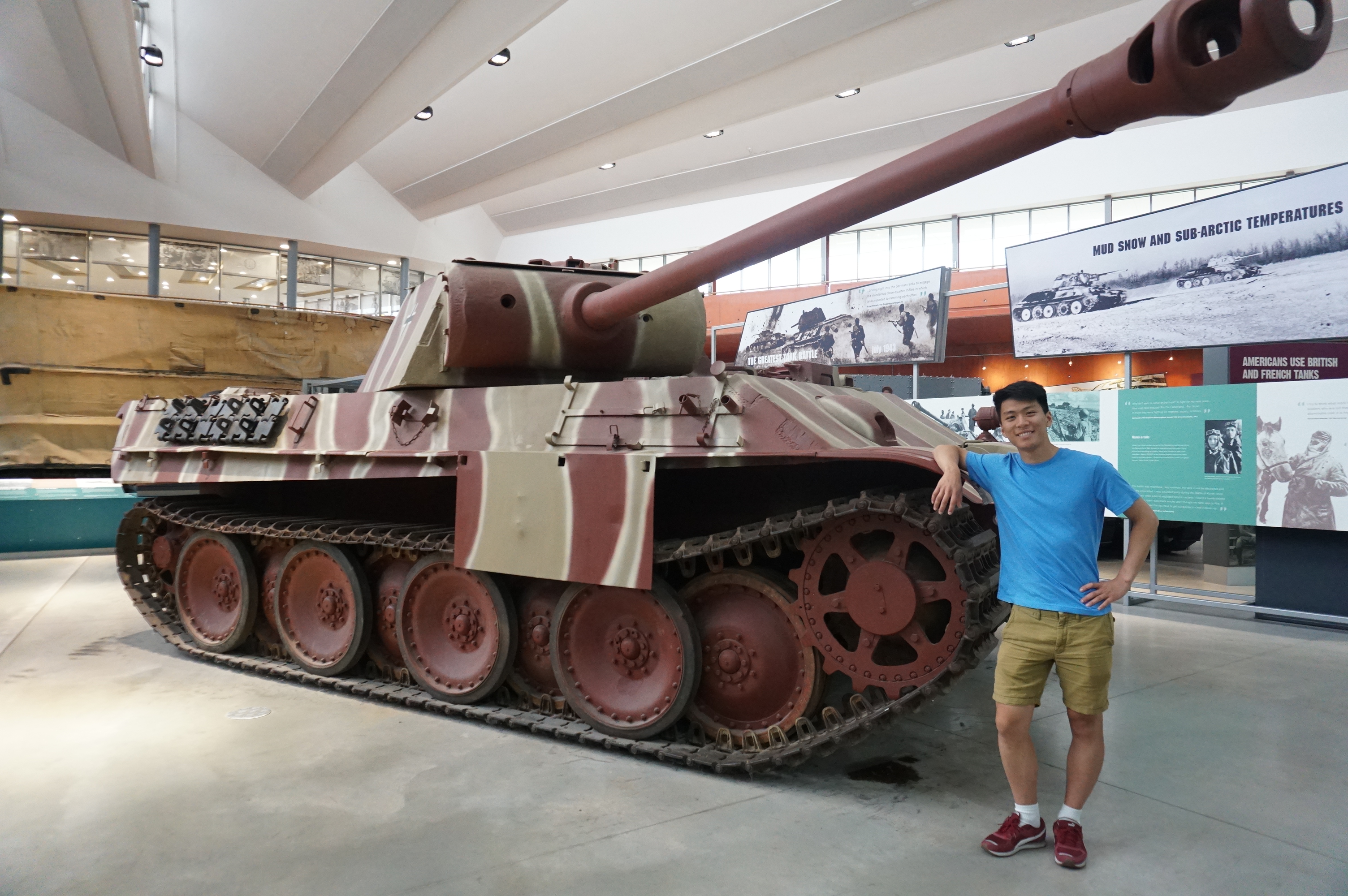
In the summer of 1943, the Allies invaded Italy, an axis power, to try and open up another front against German-occupied mainland Europe. Here, the Allies encountered a new kind of German tank - officially designated as the Sonderkraftfahrzeug 171 ("special ordnance vehicle 171") but better known as the Panther. The Panther was substantially better armored and armed than most other tanks the Allies faced and was developed in response to the excellently-designed T-34 tanks that the Soviets fielded on the Eastern front.

Me with a Panther at the Bovington Tank Museum in Dorset, UK.

The Panther had an excellent 75 mm caliber anti-tank gun which, using its standard armor-piercing rounds, could reliably (~50% of the time) penetrate over 100 mm of steel armor from 3 km away [1]. The M4, which was the most prevalent tank fielded by the Allies, had around 90 mm of frontal armor. Most tank engagements took place well within 3 km anyways, so the advent of the Panther posed a major existential threat to Allied armor - it could, from practically any realistic engagement range, penetrate and destroy the majority of Allied tanks.

The Problem

The Panther, despite being so powerful, could only really have an impact on the war if it were fielded in significant numbers. There was thus a significant need on the Allied side to reliably estimate how many Panthers the Germans were producing. This job fell on the Economic Warfare Division of the American Embassy in London [2].

Like cars, tanks are sophisticated machines composed of many, many complex parts that are manufactured beforehand, from gearboxes to gun sights to engine blocks to road wheels. In particular, the manufacture of the Panther's gearbox (the device containing the gears and gear trains within the transmission) was done very methodically; to easily communicate repairs and the delivery of spare parts, if $N$ gearboxes were manufactured, the factory would (more or less) label them with a serial number from 1 to $N$.

As the war dragged on, and as some Panther tanks were destroyed or captured by the Allies, the analysts at the American Embassy had access the gearbox serial numbers of destroyed or captured Panthers. Assuming that these numbers were sampled randomly from the Panther population, they were then confronted with a simple question: given a selection of numbers from the sequence $1$ to $N$, how can $N$ be estimated?

A First Pass

Intuition, and I suppose some simple thoughts from probability, play a surprisingly helpful part in this problem. If, say, $N=1000$ tanks were produced in total, and the Allies knocked out $n=10$ of them and read their gearbox numbers, the largest number $k$ in the selection of $n$ would probably be somewhat close to $N$.

To get a rough feeling for the chances of this, we can do a quick napkin-sized number crunch and suppose that we are sampling with replacement. If the Allies knocked out 10 tanks, then the chances that all 10 tanks had gearbox numbers 900 or below is $0.9^{10} \approx 0.349$ (each tank has a $0.9$ chance of being below number 900, and 10 tanks are sampled, so the probability of all 10 being below number 900 is $0.9^{10}$).

The point is, if we just took $k$ to be an estimator for $N$, then only around 34.8% of the time our estimate would be far off - below 900. Equivalently, around 65.2% of the time, our estimate would be between 900 and 1000. Not bad, right? Especially in a war, if the enemy had 1000 tanks and you consistently predicted they had somewhere between 900 and 1000, you were probably doing an excellent job! All based on the gearbox numbers from 10 tanks!

But something probably bothers you - $k$ is always less than, or equal to, $N$. If we assumed $k$ were the estimator of $N$, then we would consistently be underestimating $N$. In statistics lingo you can say that the expectation value (the average value if we repeated this experiment many times) of the estimator $k$, is inaccurate.

There's a simple improvement - we just need to add a correction that shifts the expectation value of the estimator closer to $N$. Think of our total number of tanks - say, 1000 - as a long number line. When we sample randomly, we are observing certain numbers pop up on this number line. The average distance between successive observations will prove very useful: if we add the average distance to $k$, that would be a better ballpark estimate for $N$. Why? Well, if $N$ were farther from $k$ than the average distance, it would be much more likely to observe a greater $k$. If $N$ were closer, $k$ would be closer to $N$, which is more unlikely. All in all, it would be unlikely for $N$ to be significantly deviant from $k$ than the average distance!

What's the average distance? Well if we observed tanks 14 and 19, for example, their distance is 4 (the numbers 15, 16, 17, 18 are in between) and it isn't $19-14=5$ because we're sampling with replacement. So, the average distance must be

$$\frac{k-n}{n}$$

since there are $k-n$ tanks that are in between samples, and dividing that total by the number of samples must yield the average distance.

Okay, so we have an estimator! Assuming we sample $n$ tanks, with $k$ being the largest sample, we can come up with a rough estimate $\mathcal{E}$ for the total number of tanks $N$ with

$$\mathcal{E}(k) = k + \frac{k-n}{n} = k\left(1+\frac{1}{n}\right)-1 .$$

But how good is this estimate?

The First Pass Wasn't So Bad

It turns out that $\mathcal{E}$ is the best possible estimator. We could have arrived at this conclusion more rigorously via lengthy derivations - but what we have currently gives us a chance to use the Lehmann–Scheffé theorem:

any estimator which is unbiased for a given unknown quantity and that depends on the data only through a complete, sufficient statistic is the unique best unbiased estimator of that quantity [3].

In other words, if an estimator (in our case, $\mathcal{E}$) has the same expectation value (average value after we estimate many times) as the unknown quantity ($N$), and if it only depends on complete and sufficient variables ($k$), then it is the unique estimator that gives us estimates closest (lowest variance) to the real value.

Regarding the theorem, we should faithfully discuss a few things: (a) that $\mathcal{E}$ has the same expectation value as $N$ (unbiased), and that $k$ is (b) complete and (c) sufficient. I'll define complete and sufficient shortly.

(a) Unbiased-ness

Essentially this is checking that $\mathcal{E}$ has the same expectation value as $N$.

This might be unsettling to those that appreciate rigor more than I do, but the most convincing way I can think of showing this (without introducing and trying to understand a long and dry proof) is to just demonstrate it using toy data.

We can have a function that generates a sample from $N$; this is randomly "destroying" or "capturing" $n$ tanks and reading their serial numbers:

import numpy as np
def generate_selection(N, n):
    sample_array = np.random.choice(N, n, replace=False)
    return sample_array+1 # +1 because tank numbering starts at 1, not 0!

and also define another function to apply our estimator:

def estimator(sample_array):
    # just k*(1+(1/n))+1
    estimate = np.amax(sample_array)*(1+1/len(sample_array)) - 1
    return estimate

Let's keep $N=1000$, and select, say, $n=20$. We can then sample and estimate many, many times to get a feeling for what the expectation value should be (albeit for this particular configuration):

estimates = []
for j in range(100000):
    num = make_prediction(generate_selection(1000, 20))
    estimates.append(num)
print(np.mean(estimates))

> 1000.0722469999998

After doing 100,000 runs, our expectation value is pretty close to 1000!

I know this isn't a proof, but I hope it's pretty strong evidence that at least for $N=1000$ and $n=20$, $\mathcal{E}$ is unbiased. We could of course generate this same evidence for other $N$ and $n$.

(b) Completeness

So if you look in a textbook, you'll find the (textbook!) definition of completeness:

A statistic $T$ is called complete if $E(g(T))=0$ for all $\theta$ and some function $g(t)$ implies that $P_{\theta}(g(T)=0)=1$ for all $\theta$

A statistic $T$ is any number that is extracted from our sample - in our case, $k$. $E(g(T))$ is the expectation value of $g(T)$ calculated with respect to $P_{\theta}$, which is a probability distribution that's parameterized by $\theta$ - in our case, the distributions of $k$.

Now this isn't terribly illuminating, but note that for a discrete situation like ours, based on the definition of an expectation value we can write

$$ E(g(T)) = \sum_t g(t)P_{\theta}(T=t) $$

and so the definition of completeness, in the most basic terms, says that $T$ is complete if $\sum_t g(t)P_{\theta}(T=t) = 0$ implies $g(t)=0$. However, taking the sum $\sum_t g(t)P_{\theta}(T=t)$ is exactly like taking the inner product of the function $g(t)$ with the function $P_{\theta}(T=t)$. Consider these functions as vectors.

Now this is interesting, because the theorem now says that "for any function $g$, if the inner product with every $P_{\theta}$ is zero, then $g$ must be zero." If you've done some linear algebra, this should sound pretty familiar: it means that if $g$ is orthogonal to every $P_{\theta}$, then $g$ must be zero, which is another way of saying that $g$ is in the span of $P_{\theta}$. So completeness is fundamentally a notion of how much $P_\theta$ spans with regard to $T$!

Showing this conclusion for $k$ is quite involved (as far as I know) because we must write out $E(g(k))=0$ and derive the conclusion that $g(k)=0$ for some $g$. You're just going to have to take my word (or someone else's, unless you want to prove it yourself - this might help!) that $k$ is complete (for better or for worse, I don't think long proofs belong in my blog posts). My main point was to show you that completeness is a pretty cool concept.

(c) Sufficiency

Sufficiency is a little easier to understand - crudely, a statistic ($k$) is sufficient with respect to a parameter ($N$) if "no other statistic that can be calculated from the same sample provides any additional information as to the value of the parameter" [4]. It's saying that $k$ is all we need (sufficient) to estimate $N$.

This makes intuitive sense, because if our other samples (like the second-largest or third-largest serial numbers) were to change a bit, our estimation of $N$ would be just as good if $k$ remained the same. For example, if we sampled tanks 4, 6, 9, 18, and 23, then our estimate of $N$ wouldn't be helped at all if number 18 were instead number 17 or something else. In this sense, $k$ is all we need.

Hopefully you're now convinced (at least intuitively) that $k$ is also sufficient.

At the end of the day, the conclusion of the Lehmann–Scheffé is profound when applied to our problem: a one-of-a-kind, best, estimator exists, and that we found it! Through some simple reasoning and thoughtful refinements, we've come up with an estimator $\mathcal{E}$ that is literally the best estimator out there. If you're an Allied statistician, you've just generated critical pieces of wartime intelligence from a humble scrounging of data. In statistics, this kind of optimized estimator is known as a minimum-variance unbiased estimator, or MVUE - you can say that $\mathcal{E}$ is the MVUE of $N$.

Further Observations

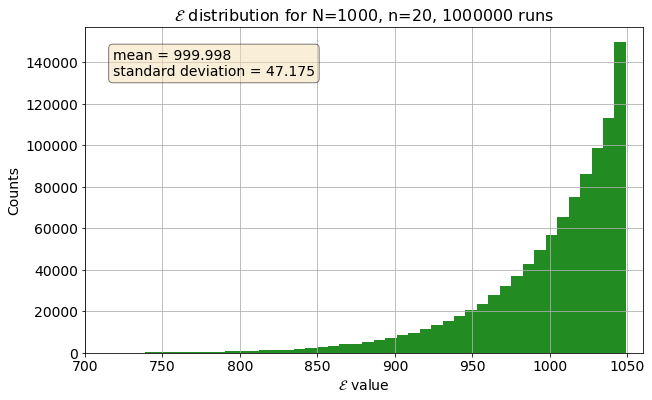
We can now explore our shiny new MVUE, and a first thing we can do is to plot the distribution of estimates with toy data. That is, if we had a sample of $N=1000$ tanks, and repeatedly drew $n=20$ many times (like a million), and then used our MVUE to estimate $N$ each time, what does the distribution of our MVUE output ($\mathcal{E}$) look like? Would it average around $1000,$ like we (obviously) expect?

Reassuringly, the mean is basically 1000. The distribution is very asymmetrical - we are much more likely to overestimate rather than underestimate $N$ by the same amount, and there seems to be an upper limit on our overestimation - we can only overestimate by around 50 tanks or so, but our underestimation can be quite bad - it is possible to underestimate by a few hundred tanks! Remember, though, that our estimate is just our highest observed element $k$ shifted by a value - so the asymmetric distribution sort of makes sense. It should resemble a shifted distribution of $k$, which should ramp up as it approaches $N$.

Undoubtedly, we'll recover similar-looking distributions from other configurations - we can easily vary the parameters of our tests, like changing $n$. A more involved study on this problem can certainly yield fancier realizations, like a quantitative measure of the uncertainty, but I think we've done a just introduction of this problem.

Final Thoughts

At the end of the day, the solution to the German Tank Problem is a systematic way to extrapolate data. To arrive here, we used some ridiculously simple reasoning that's backed up by profound ideas in probability.

So how did it turn out for the Allies [2]? As an example, for general tank production in August 1942 (okay, I know this is before the Panther was encountered, but the point still stands), the mathematical model predicted a production of 327 tanks - while intelligence (spies, radio intercepts, etc.) predicted 1550 tanks. The actual production, from records found post-war? 342.

Did I also mention how much more money, resources, and time that traditional intelligence gathering, from deploying spies to taking aerial photos, requires? In contrast the mathematical model only required some digging up of records, and perhaps some determined work at a office desk - and still produced an estimate that was orders of magnitude better!

There's a cute anecdote [5] of a situation that occurred in 1991, when an American officer was given access to view Israel's Merkava ("chariot") tank production lines; he was denied when he asked for the production number, but he "found [the denial] amusing because there was a serial number on each tank chassis."

I guess the lesson is, if you ever find yourself working as a spy, a war minister, or in a tank factory, don't forget to think about probability!

References & Further Reading

Written on July 6th, 2020 by Alex Wen
Have a suggestion or found an error? I'd be happy to know at alex.wen[at]alumni.ubc.ca.